Bootstrap Current Self-Consistency
This tutorial demonstrates how to optimize a quasi-symmetric equilibrium to have a self-consistent bootstrap current profile. This is performed by minimizing the difference between the toroidal currents \(\langle J \cdot B \rangle\) computed from the MHD equilibrium and from the Redl formula. The Redl formula is only valid in the limit of perfect quasi-symmetry, so this procedure will not work for other configurations that are not quasi-symmetric.
There are two methods that can be used, and both will be shown:
Optimize the current profile for self-consistency
Iteratively solve the equilibrium with new current profiles
These methods should be equivalent, although one might be faster than the other depending on the particular problem.
[1]:
import sys
import os

sys.path.insert(0, os.path.abspath("."))
sys.path.append(os.path.abspath("../../../"))
If you have access to a GPU, uncomment the following two lines before any DESC or JAX related imports. You should see about an order of magnitude speed improvement with only these two lines of code!
[ ]:
# from desc import set_device
# set_device("gpu")
As mentioned in DESC Documentation on performance tips, one can use compilation cache directory to reduce the compilation overhead time. Note: One needs to create jax-caches folder manually.
[3]:
# import jax

# jax.config.update("jax_compilation_cache_dir", "../jax-caches")
# jax.config.update("jax_persistent_cache_min_entry_size_bytes", -1)
# jax.config.update("jax_persistent_cache_min_compile_time_secs", 0)
[4]:
import numpy as np

np.set_printoptions(linewidth=np.inf)
import matplotlib.pyplot as plt

plt.rcParams["font.size"] = 14

from desc.compat import rescale
from desc.equilibrium import EquilibriaFamily
from desc.examples import get
from desc.grid import LinearGrid
from desc.objectives import (
    BootstrapRedlConsistency,
    FixAtomicNumber,
    FixBoundaryR,
    FixBoundaryZ,
    FixCurrent,
    FixElectronDensity,
    FixElectronTemperature,
    FixIonTemperature,
    FixPsi,
    ForceBalance,
    ObjectiveFunction,
)
from desc.plotting import plot_1d
from desc.profiles import PowerSeriesProfile, SplineProfile
As an example, we will reproduce the QA results from Landreman et al. (2022).
We will start with the “precise QA” example equilibrium, scaled to the ARIES-CS reactor size.
[5]:
eq0 = get("precise_QA")
eq0 = rescale(eq0, L=("R0", 10), B=("B0", 5.86))
This equilibrium has the vacuum profiles \(p = 0 ~\text{Pa}\) and \(\frac{2\pi}{\mu_0} I = 0 ~\text{A}\). Calculating the bootstrap current requires knowledge of the temperature and density profiles for each species in the plasma. We replace the pressure profile with the following kinetic profiles corresponding to \(\langle\beta\rangle=2.5\%\):
\(n_e = n_i = 2.38\times10^{20} (1 - \rho^{10}) ~\text{m}^{-3}\)
\(T_e = T_i = 9.45\times10^{3} (1 - \rho^{2}) ~\text{eV}\)
The temperature profiles must be given for both ions and electrons, but only the electron density profile is specified. The ion density profile is given by the effective atomic number \(Z_{eff}\) as \(n_i = n_e / Z_{eff}\). The plasma pressure will then be computed as
\(p = e (n_e T_e + n_i T_i)\).
[6]:
eq0.pressure = None  # must remove the pressure profile before setting kinetic profiles
eq0.atomic_number = PowerSeriesProfile([1])
eq0.electron_density = PowerSeriesProfile(params=[1, -1], modes=[0, 10]) * 2.38e20
eq0.electron_temperature = PowerSeriesProfile(params=[1, -1], modes=[0, 2]) * 9.45e3
eq0.ion_temperature = PowerSeriesProfile(params=[1, -1], modes=[0, 2]) * 9.45e3
# the existing current profile is the vacuum case eq0.current = PowerSeriesProfile([0])
We need to re-solve the equilibrium force balance with the new profiles.
[7]:
eq0, _ = eq0.solve(objective="force", optimizer="lsq-exact", verbose=3)
Building objective: force
Precomputing transforms
Timer: Precomputing transforms = 714 ms
Timer: Objective build = 1.69 sec
Building objective: lcfs R
Building objective: lcfs Z
Building objective: fixed Psi
Building objective: fixed current
Building objective: fixed electron density
Building objective: fixed electron temperature
Building objective: fixed ion temperature
Building objective: fixed atomic number
Building objective: fixed sheet current
Building objective: self_consistency R
Building objective: self_consistency Z
Building objective: lambda gauge
Building objective: axis R self consistency
Building objective: axis Z self consistency
Timer: Objective build = 773 ms
Timer: LinearConstraintProjection build = 6.09 sec
Number of parameters: 856
Number of objectives: 5346
Timer: Initializing the optimization = 8.71 sec

Starting optimization
Using method: lsq-exact
Solver options:
------------------------------------------------------------
Maximum Function Evaluations       : 501
Maximum Allowed Total Δx Norm      : inf
Scaled Termination                 : True
Trust Region Method                : qr
Initial Trust Radius               : 1.431e+02
Maximum Trust Radius               : inf
Minimum Trust Radius               : 2.220e-16
Trust Radius Increase Ratio        : 2.000e+00
Trust Radius Decrease Ratio        : 2.500e-01
Trust Radius Increase Threshold    : 7.500e-01
Trust Radius Decrease Threshold    : 2.500e-01
------------------------------------------------------------

   Iteration     Total nfev        Cost      Cost reduction    Step norm     Optimality
       0              1          1.138e-02                                    4.748e-02
       1              3          2.450e-03      8.927e-03      1.689e-01      1.805e-02
       2              4          1.003e-03      1.447e-03      2.762e-01      1.479e-02
       3              5          7.749e-04      2.284e-04      2.107e-01      1.472e-02
       4              6          2.205e-05      7.529e-04      5.663e-02      1.408e-03
       5              8          6.017e-06      1.603e-05      2.894e-02      6.948e-04
       6              9          3.382e-06      2.635e-06      2.959e-02      7.920e-04
       7             11          7.237e-07      2.658e-06      7.521e-03      6.954e-05
       8             12          7.116e-07      1.216e-08      1.528e-02      1.824e-04
       9             13          6.305e-07      8.108e-08      3.803e-03      1.213e-05
      10             14          6.235e-07      6.934e-09      7.823e-03      4.239e-05
      11             15          6.152e-07      8.309e-09      7.202e-03      4.238e-05
      12             16          6.104e-07      4.793e-09      7.663e-03      4.043e-05
      13             17          5.970e-07      1.342e-08      1.904e-03      2.954e-06
      14             18          5.928e-07      4.229e-09      3.800e-03      1.038e-05
Optimization terminated successfully.
`ftol` condition satisfied. (ftol=1.00e-02)
         Current function value: 5.928e-07
         Total delta_x: 6.427e-01
         Iterations: 14
         Function evaluations: 18
         Jacobian evaluations: 15
Timer: Solution time = 16.1 sec
Timer: Avg time per step = 1.07 sec
==============================================================================================================
                                                                 Start  -->   End
Total (sum of squares):                                      1.138e-02  -->   5.928e-07,
Maximum absolute Force error:                                5.309e+07  -->   1.983e+06 (N)
Minimum absolute Force error:                                1.261e+00  -->   2.978e+01 (N)
Average absolute Force error:                                5.121e+06  -->   5.254e+04 (N)
Maximum absolute Force error:                                1.512e-02  -->   5.649e-04 (normalized)
Minimum absolute Force error:                                3.591e-10  -->   8.483e-09 (normalized)
Average absolute Force error:                                1.459e-03  -->   1.496e-05 (normalized)
R boundary error:                                            0.000e+00  -->   3.846e-16 (m)
Z boundary error:                                            0.000e+00  -->   2.326e-16 (m)
Fixed Psi error:                                             0.000e+00  -->   0.000e+00 (Wb)
Fixed current profile error:                                 0.000e+00  -->   0.000e+00 (A)
Fixed electron density profile error:                        0.000e+00  -->   0.000e+00 (m^-3)
Fixed electron temperature profile error:                    0.000e+00  -->   0.000e+00 (eV)
Fixed ion temperature profile error:                         0.000e+00  -->   0.000e+00 (eV)
Fixed atomic number profile error:                           0.000e+00  -->   0.000e+00 (dimensionless)
Fixed sheet current error:                                   0.000e+00  -->   0.000e+00 (~)
==============================================================================================================
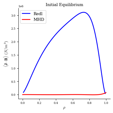
Now we have our initial equilibrium, which does not have a self-consistent bootstrap current:
[8]:
# the Redl formula is undefined at rho=0.0 and where the profiles vanish, so
# in our case here it is NaN at the axis and at rho=1.0
fig, ax = plot_1d(
    eq0,
    "<J*B> Redl",
    color="b",
    lw=2,
    label="Redl",
)
fig, ax = plot_1d(eq0, "<J*B>", color="r", lw=2, label="MHD", ax=ax)
ax.legend(loc="best")
ax.set_title("Initial Equilibrium");
/CODES/DESC/desc/utils.py:572: UserWarning: Redl formula is undefined at rho=0, but grid has grid points at rho=0, note that on-axiscurrent will be NaN.
  warnings.warn(msg, err)
/CODES/DESC/desc/utils.py:572: UserWarning: Redl formula is undefined where kinetic profiles vanish, but given electron density vanishes at at least one providedrho grid point.
  warnings.warn(msg, err)
/CODES/DESC/desc/utils.py:572: UserWarning: Redl formula is undefined where kinetic profiles vanish, but given electron temperature vanishes at at least one providedrho grid point.
  warnings.warn(msg, err)
/CODES/DESC/desc/utils.py:572: UserWarning: Redl formula is undefined where kinetic profiles vanish, but given ion temperature vanishes at at least one providedrho grid point.
  warnings.warn(msg, err)
We need to create a grid on which to evaluate the boootstrap current self-consistency. The bootstrap current is a radial profile, but the grid must have finite poloidal and toroidal resolution to accurately compute flux surface quantities. The Redl formula is undefined where the kinetic profiles vanish, so in our example we do not include points at \(\rho=0\) or \(\rho=1\).
[9]:
grid = LinearGrid(
    M=eq0.M_grid,
    N=eq0.N_grid,
    NFP=eq0.NFP,
    sym=eq0.sym,
    rho=np.linspace(1 / eq0.L_grid, 1, eq0.L_grid) - 1 / (2 * eq0.L_grid),
)
Our current profile will be represented as a power series of the form:
\(I = c_0 + c_1 \rho + c_2 \rho^2 + \mathcal{O}(\rho^3)\)
Physically, the current should vanish on the magnetic axis so \(c_0 = 0\). And in order for the MHD equilibrium to be analytic, it should scale as \(\mathcal{O}(\rho^2)\) near the magnetic axis so \(c_1 = 0\) also. However, the Redl bootstrap current formula scales as \(\mathcal{O}(\sqrt{\rho})\) near the magnetic axis. This is incorrect, because the drift-kinetic equation from the Redl formula does not account for finite orbit width effects that become important near the axis.
Typically, we use even power series with sym=True for all equilibrium profiles to give the desired analycity conditions. For bootstrap current optimizations, it is recommended to use the full power series with sym=False while also enforcing \(c_0 = c_1 = 0\). This prevents getting good self-consistency near the magnetic axis, but allows for good agreement throughout the rest of the plasma volume and results in high quality equilibria overall.
[10]:
eq0.current = PowerSeriesProfile(np.zeros((eq0.L + 1,)), sym=False)
1. Optimization
In this method, we will optimize the current profile to minimize the self-consistency errors evaluated by the BootstrapRedlConsistency objective. This objective requires the helicity, which for QA is \((M, N) = (1, 0)\).
In this example we will only optimize the current profile, so all other profiles and the plasma boundary are constrained to be fixed. It is recommended to use a very small value for gtol when optimizing the bootstrap current.
[11]:
eq1 = eq0.copy()
[12]:
objective = ObjectiveFunction(
    BootstrapRedlConsistency(eq=eq1, grid=grid, helicity=(1, 0)),
)
constraints = (
    FixAtomicNumber(eq=eq1),
    FixBoundaryR(eq=eq1),
    FixBoundaryZ(eq=eq1),
    FixCurrent(eq=eq1, indices=[0, 1]),  # fix c_0=c_1=0 current profile coefficients
    FixElectronDensity(eq=eq1),
    FixElectronTemperature(eq=eq1),
    FixIonTemperature(eq=eq1),
    FixPsi(eq=eq1),
    ForceBalance(eq=eq1),
)
eq1, _ = eq1.optimize(
    objective=objective,
    constraints=constraints,
    optimizer="proximal-lsq-exact",
    maxiter=10,
    verbose=3,
)
Building objective: Bootstrap current self-consistency (Redl)
Precomputing transforms
Timer: Precomputing transforms = 1.06 sec
Timer: Objective build = 1.94 sec
Building objective: force
Precomputing transforms
Timer: Precomputing transforms = 75.2 ms
Timer: Objective build = 136 ms
Timer: Objective build = 20.0 ms
Timer: Eq Update LinearConstraintProjection build = 3.74 sec
Timer: Proximal projection build = 19.6 sec
Building objective: fixed atomic number
Building objective: lcfs R
Building objective: lcfs Z
Building objective: fixed current
Building objective: fixed electron density
Building objective: fixed electron temperature
Building objective: fixed ion temperature
Building objective: fixed Psi
Timer: Objective build = 585 ms
Timer: LinearConstraintProjection build = 1.66 sec
Number of parameters: 7
Number of objectives: 16
Timer: Initializing the optimization = 21.9 sec

Starting optimization
Using method: proximal-lsq-exact
Solver options:
------------------------------------------------------------
Maximum Function Evaluations       : 51
Maximum Allowed Total Δx Norm      : inf
Scaled Termination                 : True
Trust Region Method                : qr
Initial Trust Radius               : 1.000e+00
Maximum Trust Radius               : inf
Minimum Trust Radius               : 2.220e-16
Trust Radius Increase Ratio        : 2.000e+00
Trust Radius Decrease Ratio        : 2.500e-01
Trust Radius Increase Threshold    : 7.500e-01
Trust Radius Decrease Threshold    : 2.500e-01
------------------------------------------------------------

   Iteration     Total nfev        Cost      Cost reduction    Step norm     Optimality
       0              1          2.763e-02                                    2.228e-01
       1              2          1.271e-04      2.751e-02      1.197e+07      1.221e-02
       2              3          4.028e-06      1.231e-04      2.418e+07      1.541e-03
       3              4          1.495e-06      2.533e-06      4.759e+07      5.865e-05
       4             30          1.495e-06      0.000e+00      0.000e+00      5.865e-05
Warning: A bad approximation caused failure to predict improvement.
         Current function value: 1.495e-06
         Total delta_x: 7.262e+07
         Iterations: 4
         Function evaluations: 30
         Jacobian evaluations: 4
Timer: Solution time = 2.02 min
Timer: Avg time per step = 24.3 sec
==============================================================================================================
                                                                 Start  -->   End
Total (sum of squares):                                      2.765e-02  -->   1.495e-06,
Maximum absolute Bootstrap current self-consistency error:   3.106e+06  -->   3.873e+04 (T A m^-2)
Minimum absolute Bootstrap current self-consistency error:   1.896e+05  -->   1.482e+01 (T A m^-2)
Average absolute Bootstrap current self-consistency error:   1.954e+06  -->   1.252e+04 (T A m^-2)
Maximum absolute Bootstrap current self-consistency error:   3.355e-01  -->   4.183e-03 (normalized)
Minimum absolute Bootstrap current self-consistency error:   2.048e-02  -->   1.601e-06 (normalized)
Average absolute Bootstrap current self-consistency error:   2.111e-01  -->   1.353e-03 (normalized)
Fixed atomic number profile error:                           0.000e+00  -->   0.000e+00 (dimensionless)
R boundary error:                                            3.846e-16  -->   1.154e-15 (m)
Z boundary error:                                            2.326e-16  -->   6.979e-16 (m)
Fixed current profile error:                                 0.000e+00  -->   0.000e+00 (A)
Fixed electron density profile error:                        0.000e+00  -->   0.000e+00 (m^-3)
Fixed electron temperature profile error:                    0.000e+00  -->   0.000e+00 (eV)
Fixed ion temperature profile error:                         0.000e+00  -->   0.000e+00 (eV)
Fixed Psi error:                                             0.000e+00  -->   0.000e+00 (Wb)
Maximum absolute Force error:                                1.983e+06  -->   1.794e+06 (N)
Minimum absolute Force error:                                2.978e+01  -->   7.962e+00 (N)
Average absolute Force error:                                5.254e+04  -->   8.691e+04 (N)
Maximum absolute Force error:                                5.649e-04  -->   5.109e-04 (normalized)
Minimum absolute Force error:                                8.483e-09  -->   2.268e-09 (normalized)
Average absolute Force error:                                1.496e-05  -->   2.475e-05 (normalized)
==============================================================================================================
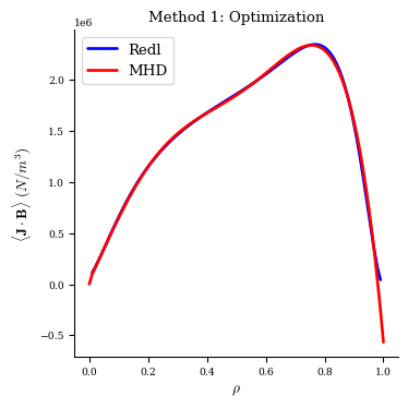
When plotting the bootstrap current profiles, we see the MHD equilibrium now has very good agreement with the Redl formula.
[13]:
fig, ax = plot_1d(eq1, "<J*B> Redl", color="b", lw=2, label="Redl")
fig, ax = plot_1d(eq1, "<J*B>", color="r", lw=2, label="MHD", ax=ax)
ax.legend(loc="best")
ax.set_title("Method 1: Optimization");
/CODES/DESC/desc/utils.py:572: UserWarning: Redl formula is undefined at rho=0, but grid has grid points at rho=0, note that on-axiscurrent will be NaN.
  warnings.warn(msg, err)
/CODES/DESC/desc/utils.py:572: UserWarning: Redl formula is undefined where kinetic profiles vanish, but given electron density vanishes at at least one providedrho grid point.
  warnings.warn(msg, err)
/CODES/DESC/desc/utils.py:572: UserWarning: Redl formula is undefined where kinetic profiles vanish, but given electron temperature vanishes at at least one providedrho grid point.
  warnings.warn(msg, err)
/CODES/DESC/desc/utils.py:572: UserWarning: Redl formula is undefined where kinetic profiles vanish, but given ion temperature vanishes at at least one providedrho grid point.
  warnings.warn(msg, err)
2. Iterative Solves
In this method, we iteratively solve the equilibrium with updated guesses for the current profile. The current profile is computed such that the parallel current is consistent with the Redl formula, according to Equation C3 in Landreman & Catto (2012). This is the same approach as STELLOPT VBOOT with SFINCS, and it usually converges in only a few iterations.
[14]:
eq2 = eq0.copy()
fam2 = EquilibriaFamily(eq2)
[15]:
niters = 3
for k in range(niters):
    eq2 = eq2.copy()
    # compute new guess for the current profile, consistent with Redl formula
    data = eq2.compute("current Redl", grid)
    current = grid.compress(data["current Redl"])
    rho = grid.compress(data["rho"])
    # fit the current profile to a power series, with c_0=c_1=0
    XX = np.fliplr(np.vander(rho, eq2.L + 1)[:, :-2])
    eq2.c_l = np.pad(np.linalg.lstsq(XX, current, rcond=None)[0], (2, 0))
    # re-solve the equilibrium
    eq2, _ = eq2.solve(objective="force", optimizer="lsq-exact", verbose=3)
    fam2.append(eq2)
Building objective: force
Precomputing transforms
Timer: Precomputing transforms = 72.1 ms
Timer: Objective build = 134 ms
Building objective: lcfs R
Building objective: lcfs Z
Building objective: fixed Psi
Building objective: fixed current
Building objective: fixed electron density
Building objective: fixed electron temperature
Building objective: fixed ion temperature
Building objective: fixed atomic number
Building objective: fixed sheet current
Building objective: self_consistency R
Building objective: self_consistency Z
Building objective: lambda gauge
Building objective: axis R self consistency
Building objective: axis Z self consistency
Timer: Objective build = 867 ms
Timer: LinearConstraintProjection build = 274 ms
Number of parameters: 856
Number of objectives: 5346
Timer: Initializing the optimization = 1.31 sec

Starting optimization
Using method: lsq-exact
Solver options:
------------------------------------------------------------
Maximum Function Evaluations       : 501
Maximum Allowed Total Δx Norm      : inf
Scaled Termination                 : True
Trust Region Method                : qr
Initial Trust Radius               : 1.498e+02
Maximum Trust Radius               : inf
Minimum Trust Radius               : 2.220e-16
Trust Radius Increase Ratio        : 2.000e+00
Trust Radius Decrease Ratio        : 2.500e-01
Trust Radius Increase Threshold    : 7.500e-01
Trust Radius Decrease Threshold    : 2.500e-01
------------------------------------------------------------

   Iteration     Total nfev        Cost      Cost reduction    Step norm     Optimality
       0              1          7.104e-03                                    8.999e-02
       1              2          3.466e-03      3.638e-03      2.023e-01      3.716e-02
       2              3          2.593e-04      3.206e-03      1.213e-01      8.056e-03
       3              4          1.499e-04      1.094e-04      9.481e-02      7.302e-03
       4              5          6.137e-05      8.857e-05      7.001e-02      3.921e-03
       5              6          2.461e-05      3.676e-05      5.578e-02      2.250e-03
       6              7          1.011e-05      1.450e-05      3.741e-02      1.271e-03
       7              8          8.362e-06      1.751e-06      3.246e-02      1.128e-03
       8              9          3.437e-06      4.926e-06      8.517e-03      1.869e-04
       9             10          3.406e-06      3.016e-08      1.767e-02      1.875e-04
      10             11          3.088e-06      3.187e-07      4.356e-03      7.847e-05
      11             12          3.021e-06      6.629e-08      4.618e-03      2.987e-05
      12             14          3.002e-06      1.981e-08      1.159e-03      8.202e-06
Optimization terminated successfully.
`ftol` condition satisfied. (ftol=1.00e-02)
         Current function value: 3.002e-06
         Total delta_x: 2.363e-01
         Iterations: 12
         Function evaluations: 14
         Jacobian evaluations: 13
Timer: Solution time = 3.99 sec
Timer: Avg time per step = 307 ms
==============================================================================================================
                                                                 Start  -->   End
Total (sum of squares):                                      7.104e-03  -->   3.002e-06,
Maximum absolute Force error:                                5.166e+07  -->   2.331e+06 (N)
Minimum absolute Force error:                                8.443e+01  -->   4.092e+00 (N)
Average absolute Force error:                                4.441e+06  -->   1.062e+05 (N)
Maximum absolute Force error:                                1.471e-02  -->   6.639e-04 (normalized)
Minimum absolute Force error:                                2.405e-08  -->   1.165e-09 (normalized)
Average absolute Force error:                                1.265e-03  -->   3.026e-05 (normalized)
R boundary error:                                            0.000e+00  -->   3.846e-16 (m)
Z boundary error:                                            0.000e+00  -->   2.326e-16 (m)
Fixed Psi error:                                             0.000e+00  -->   0.000e+00 (Wb)
Fixed current profile error:                                 0.000e+00  -->   6.664e-08 (A)
Fixed electron density profile error:                        0.000e+00  -->   0.000e+00 (m^-3)
Fixed electron temperature profile error:                    0.000e+00  -->   0.000e+00 (eV)
Fixed ion temperature profile error:                         0.000e+00  -->   0.000e+00 (eV)
Fixed atomic number profile error:                           0.000e+00  -->   0.000e+00 (dimensionless)
Fixed sheet current error:                                   0.000e+00  -->   0.000e+00 (~)
==============================================================================================================

Building objective: force
Precomputing transforms
Timer: Precomputing transforms = 66.8 ms
Timer: Objective build = 131 ms
Building objective: lcfs R
Building objective: lcfs Z
Building objective: fixed Psi
Building objective: fixed current
Building objective: fixed electron density
Building objective: fixed electron temperature
Building objective: fixed ion temperature
Building objective: fixed atomic number
Building objective: fixed sheet current
Building objective: self_consistency R
Building objective: self_consistency Z
Building objective: lambda gauge
Building objective: axis R self consistency
Building objective: axis Z self consistency
Timer: Objective build = 743 ms
Timer: LinearConstraintProjection build = 167 ms
Number of parameters: 856
Number of objectives: 5346
Timer: Initializing the optimization = 1.06 sec

Starting optimization
Using method: lsq-exact
Solver options:
------------------------------------------------------------
Maximum Function Evaluations       : 501
Maximum Allowed Total Δx Norm      : inf
Scaled Termination                 : True
Trust Region Method                : qr
Initial Trust Radius               : 1.514e+02
Maximum Trust Radius               : inf
Minimum Trust Radius               : 2.220e-16
Trust Radius Increase Ratio        : 2.000e+00
Trust Radius Decrease Ratio        : 2.500e-01
Trust Radius Increase Threshold    : 7.500e-01
Trust Radius Decrease Threshold    : 2.500e-01
------------------------------------------------------------

   Iteration     Total nfev        Cost      Cost reduction    Step norm     Optimality
       0              1          5.842e-04                                    2.129e-02
       1              2          1.374e-05      5.704e-04      6.550e-02      2.012e-03
       2              3          2.646e-06      1.109e-05      2.354e-02      3.305e-04
       3              5          1.938e-06      7.084e-07      8.600e-03      6.146e-05
       4              7          1.904e-06      3.454e-08      4.618e-03      4.600e-05
       5              8          1.890e-06      1.359e-08      4.210e-03      1.932e-05
Optimization terminated successfully.
`ftol` condition satisfied. (ftol=1.00e-02)
         Current function value: 1.890e-06
         Total delta_x: 6.890e-02
         Iterations: 5
         Function evaluations: 8
         Jacobian evaluations: 6
Timer: Solution time = 1.96 sec
Timer: Avg time per step = 326 ms
==============================================================================================================
                                                                 Start  -->   End
Total (sum of squares):                                      5.842e-04  -->   1.890e-06,
Maximum absolute Force error:                                1.265e+07  -->   1.473e+06 (N)
Minimum absolute Force error:                                5.030e+02  -->   6.140e+00 (N)
Average absolute Force error:                                1.293e+06  -->   8.187e+04 (N)
Maximum absolute Force error:                                3.602e-03  -->   4.196e-04 (normalized)
Minimum absolute Force error:                                1.433e-07  -->   1.749e-09 (normalized)
Average absolute Force error:                                3.683e-04  -->   2.332e-05 (normalized)
R boundary error:                                            0.000e+00  -->   1.781e-15 (m)
Z boundary error:                                            0.000e+00  -->   2.577e-17 (m)
Fixed Psi error:                                             0.000e+00  -->   0.000e+00 (Wb)
Fixed current profile error:                                 0.000e+00  -->   0.000e+00 (A)
Fixed electron density profile error:                        0.000e+00  -->   0.000e+00 (m^-3)
Fixed electron temperature profile error:                    0.000e+00  -->   0.000e+00 (eV)
Fixed ion temperature profile error:                         0.000e+00  -->   0.000e+00 (eV)
Fixed atomic number profile error:                           0.000e+00  -->   0.000e+00 (dimensionless)
Fixed sheet current error:                                   0.000e+00  -->   0.000e+00 (~)
==============================================================================================================

Building objective: force
Precomputing transforms
Timer: Precomputing transforms = 73.7 ms
Timer: Objective build = 134 ms
Building objective: lcfs R
Building objective: lcfs Z
Building objective: fixed Psi
Building objective: fixed current
Building objective: fixed electron density
Building objective: fixed electron temperature
Building objective: fixed ion temperature
Building objective: fixed atomic number
Building objective: fixed sheet current
Building objective: self_consistency R
Building objective: self_consistency Z
Building objective: lambda gauge
Building objective: axis R self consistency
Building objective: axis Z self consistency
Timer: Objective build = 732 ms
Timer: LinearConstraintProjection build = 182 ms
Number of parameters: 856
Number of objectives: 5346
Timer: Initializing the optimization = 1.06 sec

Starting optimization
Using method: lsq-exact
Solver options:
------------------------------------------------------------
Maximum Function Evaluations       : 501
Maximum Allowed Total Δx Norm      : inf
Scaled Termination                 : True
Trust Region Method                : qr
Initial Trust Radius               : 1.497e+02
Maximum Trust Radius               : inf
Minimum Trust Radius               : 2.220e-16
Trust Radius Increase Ratio        : 2.000e+00
Trust Radius Decrease Ratio        : 2.500e-01
Trust Radius Increase Threshold    : 7.500e-01
Trust Radius Decrease Threshold    : 2.500e-01
------------------------------------------------------------

   Iteration     Total nfev        Cost      Cost reduction    Step norm     Optimality
       0              1          2.391e-05                                    4.060e-03
       1              2          6.116e-06      1.780e-05      3.606e-02      7.476e-04
       2              3          1.856e-06      4.260e-06      1.124e-02      1.048e-04
       3              5          1.806e-06      5.084e-08      4.381e-03      2.417e-05
       4              7          1.800e-06      5.525e-09      2.266e-03      5.050e-06
Optimization terminated successfully.
`ftol` condition satisfied. (ftol=1.00e-02)
         Current function value: 1.800e-06
         Total delta_x: 4.496e-02
         Iterations: 4
         Function evaluations: 7
         Jacobian evaluations: 5
Timer: Solution time = 1.66 sec
Timer: Avg time per step = 332 ms
==============================================================================================================
                                                                 Start  -->   End
Total (sum of squares):                                      2.391e-05  -->   1.800e-06,
Maximum absolute Force error:                                3.586e+06  -->   1.489e+06 (N)
Minimum absolute Force error:                                9.634e+01  -->   4.893e+00 (N)
Average absolute Force error:                                2.651e+05  -->   8.232e+04 (N)
Maximum absolute Force error:                                1.021e-03  -->   4.240e-04 (normalized)
Minimum absolute Force error:                                2.744e-08  -->   1.394e-09 (normalized)
Average absolute Force error:                                7.550e-05  -->   2.344e-05 (normalized)
R boundary error:                                            0.000e+00  -->   1.781e-15 (m)
Z boundary error:                                            0.000e+00  -->   2.571e-17 (m)
Fixed Psi error:                                             0.000e+00  -->   0.000e+00 (Wb)
Fixed current profile error:                                 0.000e+00  -->   4.165e-09 (A)
Fixed electron density profile error:                        0.000e+00  -->   0.000e+00 (m^-3)
Fixed electron temperature profile error:                    0.000e+00  -->   0.000e+00 (eV)
Fixed ion temperature profile error:                         0.000e+00  -->   0.000e+00 (eV)
Fixed atomic number profile error:                           0.000e+00  -->   0.000e+00 (dimensionless)
Fixed sheet current error:                                   0.000e+00  -->   0.000e+00 (~)
==============================================================================================================
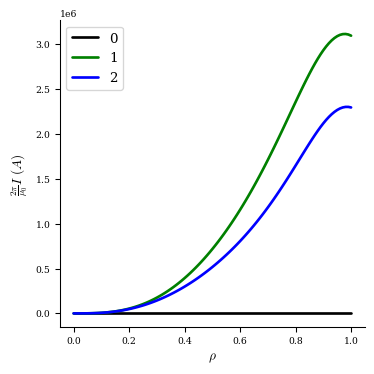
We can plot the current profile at each iteration to visualize how it changed:
[16]:
fig, ax = plot_1d(fam2[0], "current", color="k", lw=2, label="0")
fig, ax = plot_1d(fam2[1], "current", color="g", lw=2, label="1", ax=ax)
fig, ax = plot_1d(fam2[2], "current", color="b", lw=2, label="2", ax=ax)
fig, ax = plot_1d(fam2[3], "current", color="r", lw=2, label="3", ax=ax)
ax.legend(loc="best");
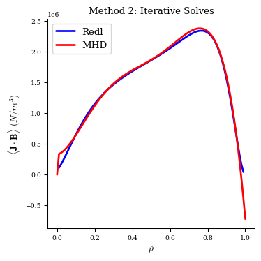
With this method the MHD equilibrium also has very good agreement with the Redl formula.
[17]:
fig, ax = plot_1d(eq2, "<J*B> Redl", color="b", lw=2, label="Redl")
fig, ax = plot_1d(eq2, "<J*B>", color="r", lw=2, label="MHD", ax=ax)
ax.legend(loc="best")
ax.set_title("Method 2: Iterative Solves");
/CODES/DESC/desc/utils.py:572: UserWarning: Redl formula is undefined at rho=0, but grid has grid points at rho=0, note that on-axiscurrent will be NaN.
  warnings.warn(msg, err)
/CODES/DESC/desc/utils.py:572: UserWarning: Redl formula is undefined where kinetic profiles vanish, but given electron density vanishes at at least one providedrho grid point.
  warnings.warn(msg, err)
/CODES/DESC/desc/utils.py:572: UserWarning: Redl formula is undefined where kinetic profiles vanish, but given electron temperature vanishes at at least one providedrho grid point.
  warnings.warn(msg, err)
/CODES/DESC/desc/utils.py:572: UserWarning: Redl formula is undefined where kinetic profiles vanish, but given ion temperature vanishes at at least one providedrho grid point.
  warnings.warn(msg, err)
Comparison
Even though both methods give good self-consistency for the bootstrap current, they do result in slightly different coefficients for the current profile:
[18]:
print(eq1.c_l)
print(eq2.c_l)
[ 0.00000000e+00  0.00000000e+00  1.15112878e+04  6.29171559e+06  3.58272704e+06 -3.59527414e+07  5.57512420e+07 -2.86198850e+07  1.35489797e+06]
[ 0.00000000e+00  0.00000000e+00  4.66585405e+05  5.63752557e+05  3.00704695e+07 -9.56770096e+07  1.26451711e+08 -7.04331552e+07  1.09842316e+07]
In this example, the first method of optimization gave better self-consistency but was noticeably slower than the second method of iterative solves.
Using Spline Profiles
We can also use splines to describe the current profile. Due to the many DOFs of splines and their local nature, they can be difficult to use with the first method shown above. So, we recommend using the iterative solve method if a spline current profile is desired.
The code for the iterative method with splines is slightly different, as now we do not need to re-fit the current profile with a power series in order to update our spline. Instead, we choose our spline profile knots carefully to include a knot at the axis which we will keep at 0 (in order to enforce zero on-axis net toroidal current), and choosing the rest to align with the grid we will be computing the Redl bootstrap current at.
Remember that the Redl formula is not defined on-axis or on the boundary, so we must ensure we do not include a knot at \(\rho=1\), as we have no way of updating that value.
[19]:
# Choose a denser grid for the spline profile so we can represent the bootstrap current profile well
L_grid = 25

grid = LinearGrid(
    M=eq0.M_grid,
    N=eq0.N_grid,
    NFP=eq0.NFP,
    sym=eq0.sym,
    rho=np.linspace(1 / L_grid, 1, L_grid) - 1 / (2 * L_grid),
)

eq2_spline = eq0.copy()
fam2 = EquilibriaFamily(eq2_spline)
# choose the rho values for the knots
rho = np.concatenate([np.array([0.0]), grid.nodes[grid.unique_rho_idx, 0]])
# make a SplineProfile for current, initially zero.
eq2_spline.current = SplineProfile(values=np.zeros_like(rho), knots=rho)
[20]:
from desc.backend import jnp

niters = 3
for k in range(niters):
    eq2_spline = eq2_spline.copy()
    # compute new guess for the current profile, consistent with Redl formula
    data = eq2_spline.compute("current Redl", grid)
    current = grid.compress(data["current Redl"])
    rho = grid.compress(data["rho"])
    # add the rho=0 value which we enforce as zero current
    c_at_knots = np.concatenate([np.array([0.0]), current])
    eq2_spline.current.params = c_at_knots
    # re-solve the equilibrium
    eq2_spline, _ = eq2_spline.solve(
        objective="force", optimizer="lsq-exact", verbose=3
    )
    fam2.append(eq2_spline)
Building objective: force
Precomputing transforms
Timer: Precomputing transforms = 90.9 ms
Timer: Objective build = 153 ms
Building objective: lcfs R
Building objective: lcfs Z
Building objective: fixed Psi
Building objective: fixed current
Building objective: fixed electron density
Building objective: fixed electron temperature
Building objective: fixed ion temperature
Building objective: fixed atomic number
Building objective: fixed sheet current
Building objective: self_consistency R
Building objective: self_consistency Z
Building objective: lambda gauge
Building objective: axis R self consistency
Building objective: axis Z self consistency
Timer: Objective build = 893 ms
Timer: LinearConstraintProjection build = 4.22 sec
Number of parameters: 856
Number of objectives: 5346
Timer: Initializing the optimization = 5.36 sec

Starting optimization
Using method: lsq-exact
Solver options:
------------------------------------------------------------
Maximum Function Evaluations       : 501
Maximum Allowed Total Δx Norm      : inf
Scaled Termination                 : True
Trust Region Method                : qr
Initial Trust Radius               : 1.498e+02
Maximum Trust Radius               : inf
Minimum Trust Radius               : 2.220e-16
Trust Radius Increase Ratio        : 2.000e+00
Trust Radius Decrease Ratio        : 2.500e-01
Trust Radius Increase Threshold    : 7.500e-01
Trust Radius Decrease Threshold    : 2.500e-01
------------------------------------------------------------

   Iteration     Total nfev        Cost      Cost reduction    Step norm     Optimality
       0              1          7.098e-03                                    9.004e-02
       1              2          4.884e-03      2.214e-03      2.084e-01      4.057e-02
       2              3          3.192e-04      4.564e-03      1.226e-01      8.920e-03
       3              4          2.414e-04      7.784e-05      1.060e-01      8.235e-03
       4              5          4.900e-06      2.365e-04      2.610e-02      3.733e-04
       5              7          2.996e-06      1.904e-06      1.485e-02      1.100e-04
       6              9          2.819e-06      1.771e-07      6.102e-03      5.988e-05
       7             11          2.761e-06      5.803e-08      3.671e-03      1.419e-05
       8             12          2.721e-06      4.015e-08      6.525e-03      3.824e-05
       9             13          2.707e-06      1.398e-08      1.187e-02      1.058e-04
      10             14          2.629e-06      7.797e-08      3.109e-03      5.613e-06
      11             15          2.614e-06      1.448e-08      5.635e-03      2.405e-05
Optimization terminated successfully.
`ftol` condition satisfied. (ftol=1.00e-02)
         Current function value: 2.614e-06
         Total delta_x: 2.312e-01
         Iterations: 11
         Function evaluations: 15
         Jacobian evaluations: 12
Timer: Solution time = 16.7 sec
Timer: Avg time per step = 1.39 sec
==============================================================================================================
                                                                 Start  -->   End
Total (sum of squares):                                      7.098e-03  -->   2.614e-06,
Maximum absolute Force error:                                5.134e+07  -->   2.062e+06 (N)
Minimum absolute Force error:                                6.833e+01  -->   1.635e+01 (N)
Average absolute Force error:                                4.425e+06  -->   1.033e+05 (N)
Maximum absolute Force error:                                1.462e-02  -->   5.872e-04 (normalized)
Minimum absolute Force error:                                1.946e-08  -->   4.657e-09 (normalized)
Average absolute Force error:                                1.260e-03  -->   2.941e-05 (normalized)
R boundary error:                                            0.000e+00  -->   3.846e-16 (m)
Z boundary error:                                            0.000e+00  -->   2.326e-16 (m)
Fixed Psi error:                                             0.000e+00  -->   0.000e+00 (Wb)
Fixed current profile error:                                 0.000e+00  -->   4.800e-10 (A)
Fixed electron density profile error:                        0.000e+00  -->   0.000e+00 (m^-3)
Fixed electron temperature profile error:                    0.000e+00  -->   0.000e+00 (eV)
Fixed ion temperature profile error:                         0.000e+00  -->   0.000e+00 (eV)
Fixed atomic number profile error:                           0.000e+00  -->   0.000e+00 (dimensionless)
Fixed sheet current error:                                   0.000e+00  -->   0.000e+00 (~)
==============================================================================================================

Building objective: force
Precomputing transforms
Timer: Precomputing transforms = 74.6 ms
Timer: Objective build = 137 ms
Building objective: lcfs R
Building objective: lcfs Z
Building objective: fixed Psi
Building objective: fixed current
Building objective: fixed electron density
Building objective: fixed electron temperature
Building objective: fixed ion temperature
Building objective: fixed atomic number
Building objective: fixed sheet current
Building objective: self_consistency R
Building objective: self_consistency Z
Building objective: lambda gauge
Building objective: axis R self consistency
Building objective: axis Z self consistency
Timer: Objective build = 740 ms
Timer: LinearConstraintProjection build = 168 ms
Number of parameters: 856
Number of objectives: 5346
Timer: Initializing the optimization = 1.06 sec

Starting optimization
Using method: lsq-exact
Solver options:
------------------------------------------------------------
Maximum Function Evaluations       : 501
Maximum Allowed Total Δx Norm      : inf
Scaled Termination                 : True
Trust Region Method                : qr
Initial Trust Radius               : 1.488e+02
Maximum Trust Radius               : inf
Minimum Trust Radius               : 2.220e-16
Trust Radius Increase Ratio        : 2.000e+00
Trust Radius Decrease Ratio        : 2.500e-01
Trust Radius Increase Threshold    : 7.500e-01
Trust Radius Decrease Threshold    : 2.500e-01
------------------------------------------------------------

   Iteration     Total nfev        Cost      Cost reduction    Step norm     Optimality
       0              1          5.723e-04                                    2.144e-02
       1              2          1.125e-05      5.611e-04      6.481e-02      1.773e-03
       2              3          2.081e-06      9.168e-06      1.462e-02      1.189e-04
       3              4          2.052e-06      2.892e-08      1.242e-02      9.357e-05
       4              6          1.983e-06      6.916e-08      3.906e-03      3.394e-05
       5              7          1.976e-06      6.929e-09      7.107e-03      2.043e-05
Optimization terminated successfully.
`ftol` condition satisfied. (ftol=1.00e-02)
         Current function value: 1.976e-06
         Total delta_x: 7.030e-02
         Iterations: 5
         Function evaluations: 7
         Jacobian evaluations: 6
Timer: Solution time = 1.66 sec
Timer: Avg time per step = 278 ms
==============================================================================================================
                                                                 Start  -->   End
Total (sum of squares):                                      5.723e-04  -->   1.976e-06,
Maximum absolute Force error:                                1.335e+07  -->   2.315e+06 (N)
Minimum absolute Force error:                                6.304e+01  -->   7.764e-01 (N)
Average absolute Force error:                                1.293e+06  -->   8.724e+04 (N)
Maximum absolute Force error:                                3.801e-03  -->   6.593e-04 (normalized)
Minimum absolute Force error:                                1.795e-08  -->   2.211e-10 (normalized)
Average absolute Force error:                                3.683e-04  -->   2.485e-05 (normalized)
R boundary error:                                            0.000e+00  -->   1.781e-15 (m)
Z boundary error:                                            0.000e+00  -->   2.577e-17 (m)
Fixed Psi error:                                             0.000e+00  -->   0.000e+00 (Wb)
Fixed current profile error:                                 0.000e+00  -->   2.671e-10 (A)
Fixed electron density profile error:                        0.000e+00  -->   0.000e+00 (m^-3)
Fixed electron temperature profile error:                    0.000e+00  -->   0.000e+00 (eV)
Fixed ion temperature profile error:                         0.000e+00  -->   0.000e+00 (eV)
Fixed atomic number profile error:                           0.000e+00  -->   0.000e+00 (dimensionless)
Fixed sheet current error:                                   0.000e+00  -->   0.000e+00 (~)
==============================================================================================================

Building objective: force
Precomputing transforms
Timer: Precomputing transforms = 76.6 ms
Timer: Objective build = 137 ms
Building objective: lcfs R
Building objective: lcfs Z
Building objective: fixed Psi
Building objective: fixed current
Building objective: fixed electron density
Building objective: fixed electron temperature
Building objective: fixed ion temperature
Building objective: fixed atomic number
Building objective: fixed sheet current
Building objective: self_consistency R
Building objective: self_consistency Z
Building objective: lambda gauge
Building objective: axis R self consistency
Building objective: axis Z self consistency
Timer: Objective build = 730 ms
Timer: LinearConstraintProjection build = 163 ms
Number of parameters: 856
Number of objectives: 5346
Timer: Initializing the optimization = 1.04 sec

Starting optimization
Using method: lsq-exact
Solver options:
------------------------------------------------------------
Maximum Function Evaluations       : 501
Maximum Allowed Total Δx Norm      : inf
Scaled Termination                 : True
Trust Region Method                : qr
Initial Trust Radius               : 1.464e+02
Maximum Trust Radius               : inf
Minimum Trust Radius               : 2.220e-16
Trust Radius Increase Ratio        : 2.000e+00
Trust Radius Decrease Ratio        : 2.500e-01
Trust Radius Increase Threshold    : 7.500e-01
Trust Radius Decrease Threshold    : 2.500e-01
------------------------------------------------------------

   Iteration     Total nfev        Cost      Cost reduction    Step norm     Optimality
       0              1          2.632e-05                                    4.461e-03
       1              2          2.064e-06      2.426e-05      1.606e-02      1.069e-04
       2              3          2.031e-06      3.265e-08      1.021e-02      7.220e-05
       3              5          1.989e-06      4.186e-08      3.607e-03      2.415e-05
       4              6          1.986e-06      3.878e-09      5.739e-03      2.184e-05
Optimization terminated successfully.
`ftol` condition satisfied. (ftol=1.00e-02)
         Current function value: 1.986e-06
         Total delta_x: 2.328e-02
         Iterations: 4
         Function evaluations: 6
         Jacobian evaluations: 5
Timer: Solution time = 1.47 sec
Timer: Avg time per step = 295 ms
==============================================================================================================
                                                                 Start  -->   End
Total (sum of squares):                                      2.632e-05  -->   1.986e-06,
Maximum absolute Force error:                                2.524e+06  -->   2.346e+06 (N)
Minimum absolute Force error:                                5.917e+01  -->   4.723e+01 (N)
Average absolute Force error:                                2.785e+05  -->   8.965e+04 (N)
Maximum absolute Force error:                                7.188e-04  -->   6.680e-04 (normalized)
Minimum absolute Force error:                                1.685e-08  -->   1.345e-08 (normalized)
Average absolute Force error:                                7.933e-05  -->   2.553e-05 (normalized)
R boundary error:                                            0.000e+00  -->   1.781e-15 (m)
Z boundary error:                                            0.000e+00  -->   2.571e-17 (m)
Fixed Psi error:                                             0.000e+00  -->   0.000e+00 (Wb)
Fixed current profile error:                                 0.000e+00  -->   5.468e-10 (A)
Fixed electron density profile error:                        0.000e+00  -->   0.000e+00 (m^-3)
Fixed electron temperature profile error:                    0.000e+00  -->   0.000e+00 (eV)
Fixed ion temperature profile error:                         0.000e+00  -->   0.000e+00 (eV)
Fixed atomic number profile error:                           0.000e+00  -->   0.000e+00 (dimensionless)
Fixed sheet current error:                                   0.000e+00  -->   0.000e+00 (~)
==============================================================================================================
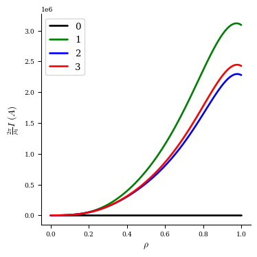
We can plot the current profile at each iteration to visualize how it changed:
[21]:
fig, ax = plot_1d(fam2[0], "current", color="k", lw=2, label="0")
fig, ax = plot_1d(fam2[1], "current", color="g", lw=2, label="1", ax=ax)
fig, ax = plot_1d(fam2[2], "current", color="b", lw=2, label="2", ax=ax)
ax.legend(loc="best");
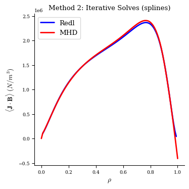
With this method the MHD equilibrium also has very good agreement with the Redl formula, now with a SplineProfile.
[22]:
fig, ax = plot_1d(fam2[-1], "<J*B> Redl", color="b", lw=2, label="Redl")
fig, ax = plot_1d(fam2[-1], "<J*B>", color="r", lw=2, label="MHD", ax=ax)
ax.legend(loc="best")
ax.set_title("Method 2: Iterative Solves (splines)");
/CODES/DESC/desc/utils.py:572: UserWarning: Redl formula is undefined at rho=0, but grid has grid points at rho=0, note that on-axiscurrent will be NaN.
  warnings.warn(msg, err)
/CODES/DESC/desc/utils.py:572: UserWarning: Redl formula is undefined where kinetic profiles vanish, but given electron density vanishes at at least one providedrho grid point.
  warnings.warn(msg, err)
/CODES/DESC/desc/utils.py:572: UserWarning: Redl formula is undefined where kinetic profiles vanish, but given electron temperature vanishes at at least one providedrho grid point.
  warnings.warn(msg, err)
/CODES/DESC/desc/utils.py:572: UserWarning: Redl formula is undefined where kinetic profiles vanish, but given ion temperature vanishes at at least one providedrho grid point.
  warnings.warn(msg, err)